
Cleaning California Public Enrollment Data

During this cleaning I discover the Caifornia Deparment of Education (CDE) doesn’t keep track of closed schools after some time. Since 1981, over 1000 schools have been forgotten. If you look at the national data, it is even worse. This seems a shame for people who attended those forgotten schools.
I was able to recover over 95% of these missing schools. The resulting dataset is publicly available for other analysts on Tableau.
I recently read a helpful article by John Sullivan on skills to showcase for a career in data science. He describes data cleaning as requiring these skills:
Since 1981, over 1000 schools have been forgotten.
In order to prepare enrollment data for analysis, I perform many of the cleaning tasks outlined above. I merge yearly enrollment, english learner, free/reduced priced lunch, public/charter, and performance data to visualize trends over time. My cleaning steps are documented in this post.
Import
Download Files
Originally I wrote a scraper in python to bulk download the files from http://www.cde.ca.gov/ds/sd/sd/, however I was having timeout issues from the cde server and clicking a few dozen links isn’t that bad, so I downloaded by hand. File formats include .csv, .xls, .txt, .zip, .dbf, .exe (all pretty straightforward except that on mac .dbf requires OpenOffice and .exe are self-extracting zip files that can be unzipped on the command line). I convert all files to either .txt or .csv and organize the files in a Data/ subdirectory within the project directory.
Import Files
In this case I import files directly from a local repository. For the most part this only requires the read.table function from base R. .txt are tab delimeted and .csv are comma delimited so the main difference is the sep parameter:
For .txt files
DT.list <- lapply(file.list, read.table, fill=TRUE, na.strings=c("", "NA"), sep ="\t", quote = "", header=TRUE, check.names=FALSE)
For .csv there is a built-in read.csv that makes sep=”,”
DT.list <- lapply(file.list, read.csv, header=TRUE, check.names=FALSE)
File Lists
I use naming conventions to differentiate files with slightly different structure that need to be modifed in order to combine them into a single data table. Then I use regex to collect files of similar type into file lists. I use lapply to perform read.table on all of the files and put the resulting data frames in a list. Each list of data frames is named by year and actions are performed on their columns en masse.
For example, with the EL data that was in .csv format we find that ‘80 contained a duplicate CDS_CODE column that needed to be removed. Notice that I remove that column before renaming all of the columns and combining the data frames into one data table with rbindlist from the data.table package.
#Convert file list into a data.table with an ID row (Using starting year as the year indicator)
DT.list <- lapply(el8000.list, read.csv, header=TRUE, check.names=FALSE)
setattr(DT.list, 'names', c("1980", "1981", "1982","1983", "1984", "1985", "1986", "1987", "1988", "1989", "1990", "1991", "1992", "1993", "1994", "1995", "1996", "1997", "1998", "1999", "2000"))
DT.list$`1980`$'CDS_CODE,C,14' <- NULL # Remove duplicate CDS col from 1980
DT.list <- lapply(DT.list, setNames, colnames)
DT00 <- rbindlist(DT.list, use.names=TRUE, fill=TRUE, idcol='YEAR') # creates data.table from list of data.frames
Join
rbindlist is significantly faster than rbind, so ideally we can modify our list of dataframes and create one long list before our call to rbindlist. This requires that each dataframe have the same structure (number of variables, colnames, coltypes). When unable to put all of the data frames in one list, I use rbind to bind the rows of the data tables.
CDE does include a file structure file for each individual file, so I look through these to find some structural changes to the data. At times these structure files are incomplete or incorrect.
Enrollment
With enrollment data, structural changes create 5 timespans: 1981-1992, 1993-1997, 1998-2006, 2007-2008, 2009-2017. The primary difference is that ETHNIC categories change as discussed in my post on Enrollments by Ethnicity. Additionally there are historical enrollment files from 1948-1980, however they don’t include many variables. 1948-1969 seperate grades and gender, 1970-1976 seperate gender, 1977-1980 only have county-level enrollment (no School-level data, no ethinicities).
CDS_CODE
County, District, and School values are missing from 1981-1992, 1993-1997, and 2007-2008, so these are imputed with correct values from a database of California Public Schools.
#Load database of California Public Schools
#CDE doesn't keep complete CDS records at https://www.cde.ca.gov/ds/si/ds/pubschls.asp
pubsch <- read.table("./Data/CA/pubschls.txt", fill=TRUE, na.strings=c("", "NA"), sep ="\t", quote = "", header=TRUE)
pubsch <- data.table(pubsch)
setnames(pubsch, c("CDSCode", "County", "District", "School"), c("CDS_CODE", "COUNTY", "DISTRICT", "SCHOOL"))
pubsch <- pubsch[, CDS_CODE:=as.character(CDS_CODE)]
#Attempted NCES list at https://nces.ed.gov/programs/edge/geographicGeocode.aspx but it was LESS schools

#Create data.table with CDSCode County District School Charter Latitude Longitude
sch <- pubsch[,.(CDS_CODE, COUNTY, DISTRICT, SCHOOL, Charter, Latitude, Longitude)]
setkey(sch, CDS_CODE)
sch <- unique(sch)

#Create data.table with school CDS information only
cds <- sch[,.(CDS_CODE, COUNTY, DISTRICT, SCHOOL)]
setkey(cds, CDS_CODE)

#Set key for data tables
setkey(DT92, CDS_CODE); setkey(DT06, CDS_CODE); setkey(DT97, CDS_CODE); setkey(DT16, CDS_CODE)

#Reorder cols in DT92, DT08 and DT16
setcolorder(DT08, c("CDS_CODE", "COUNTY", "DISTRICT", "SCHOOL", "YEAR", "ETHNIC", "GENDER", "KDGN", "GR_1", "GR_2", "GR_3", "GR_4", "GR_5", "GR_6", "GR_7", "GR_8", "UNGR_ELM", "GR_9", "GR_10", "GR_11", "GR_12", "UNGR_SEC", "ENR_TOTAL", "ADULT"))
setcolorder(DT16, c("CDS_CODE", "COUNTY", "DISTRICT", "SCHOOL", "YEAR", "ETHNIC", "GENDER", "KDGN", "GR_1", "GR_2", "GR_3", "GR_4", "GR_5", "GR_6", "GR_7", "GR_8", "UNGR_ELM", "GR_9", "GR_10", "GR_11", "GR_12", "UNGR_SEC", "ENR_TOTAL", "ADULT"))

#Merge County, District, School onto 92, 97 and 06 datatables
DT92 <- cds[DT92] # duplicates existing district and school
DT97 <- cds[DT97]
DT06 <- cds[DT06]
Ethnicity
Since ETHNIC categories changed I kept four timespans as seperate .csv files. Of note, the description of the ETHNIC field for the Enr81To92.txt file is incorrect, (https://www.cde.ca.gov/ds/sd/sd/fsenr81to92.asp) says:
- Code 1 = American Indian or Alaska Native
- Code 2 = Asian
- Code 3 = Pacific Islander
- Code 4 = Filipino
- Code 5 = Hispanic or Latino
- Code 6 = Black, not Hispanic
- Code 7 = White, not Hispanic
When in fact the levels of the ETHNIC field are character strings:
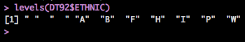
- “A” = Asian
- “B” = Black, not Hispanic
- “F” = Filipino
- “H” = Hispanic or Latino
- “I” = American Indian or Alaska Native
- “P” = Pacific Islander
- “W” = White, not Hispanic
- ” “ and “ “ = Enrollment by racial/ethnic designation was not collected during the 1982–83 and 1983–84 data collection. Therefore this field will contain blanks for these two years (when the YEAR field is equal to “8283” or “8384”).
English Larners
For ELs there is a hint about the TOTAL variable starting in 95 and changing in 98. However, changing colnames is straightforward, the full story is that the filetype changes between starting year 2000 and 2001, there are no header rows for starting years 2002-2008, and the duplicate column in ‘80 that was removed in the code snippet for file lists above.
Free/Reduced Lunch
There is a change in filetype between 2003 and 2004. In the first set there are 3 different groups of variables (1988-1997 13 variables, 1998 14 variables, 1999-2003 15 variables) a sample of the structure from the file list is shown below:
 $ 1997:'data.frame':	7966 obs. of  13 variables:
  ..$ FYR,C,9         : Factor w/ 1 level "1997/1998": 1 1 1 1 1 1 1 1 1 1 ...
  ..$ CCODE,C,2       : int [1:7966] 1 1 1 1 1 1 1 1 1 1 ...
  ..$ DCODE,C,5       : int [1:7966] 61119 61119 61119 61119 61119 61119 61119 61119 61119 61119 ...
  ..$ SCODE,C,7       : int [1:7966] 130229 132878 134304 6000004 6090005 6090013 6090021 6090039 6090047 6090054 ...
  ..$ DNAME,C,25      : Factor w/ 976 levels "ABC UNIFIED",..: 6 6 6 6 6 6 6 6 6 6 ...
  ..$ SNAME,C,30      : Factor w/ 6692 levels "A STREET ELEMENTARY",..: 40 1837 2791 1062 3474 1687 4435 2089 2417 3304 ...
  ..$ GRD_SPAN,C,5    : Factor w/ 51 levels "","01-02","01-03",..: 38 38 38 27 45 45 45 45 45 27 ...
  ..$ PUBLIC_ENR,N,9,0: int [1:7966] 1617 1302 260 559 504 366 437 259 556 803 ...
  ..$ PRIVATE_EN,N,9,0: int [1:7966] 25 43 0 20 9 2 16 5 21 7 ...
  ..$ AFDC_CNT,N,9,0  : int [1:7966] 136 169 0 97 56 23 42 39 113 45 ...
  ..$ FREE_MEALS,N,9,0: int [1:7966] 364 596 59 393 217 62 129 56 345 119 ...
  ..$ AFDC_PCT,N,9,4  : num [1:7966] 8.28 12.57 0 16.75 10.92 ...
  ..$ FREE_PCT,N,9,4  : num [1:7966] 22.2 44.3 22.7 67.9 42.3 ...
  $ 1998:'data.frame':	8115 obs. of  14 variables:
  ..$ CCODE,C,7        : int [1:8115] 1 1 1 1 1 1 1 1 1 1 ...
  ..$ DCODE,C,8        : int [1:8115] 10017 61119 61119 61119 61119 61119 61119 61119 61119 61119 ...
  ..$ SCODE,C,9        : int [1:8115] 6114896 130229 132878 134304 6000004 6090005 6090013 6090021 6090039 6090047 ...
  ..$ RANK,C,6         : int [1:8115] 1 3 3 3 2 1 1 1 1 1 ...
  ..$ PUBENROLL,N,9,0  : int [1:8115] 80 1700 1404 201 532 502 351 420 284 548 ...
  ..$ NONPUBLIC,N,10,0 : int [1:8115] 0 16 31 0 36 6 4 12 3 18 ...
  *..$ CALWORKS,N,11,0  : int [1:8115] 1 103 133 26 88 55 23 35 12 97 ...*
  ..$ FREE,N,11,0      : int [1:8115] 0 301 467 41 310 176 67 97 53 270 ...
  ..$ REDUCED,N,10,0   : int [1:8115] 0 117 174 4 107 77 14 41 19 81 ...
  *..$ MEALSTOTAL,N,14,0: int [1:8115] 0 418 641 45 417 253 81 138 72 351 ...*
  *..$ CALWORKS%,N,12,4 : num [1:8115] 0.0125 0.06 0.0927 0.1294 0.1549 ...*
  ..$ MEALS%,N,11,4    : num [1:8115] 0 0.244 0.447 0.224 0.734 ...
  ..$ SCHOOL,C,31      : Factor w/ 6842 levels "","A STREET ELEMENTARY",..: 4211 41 1875 2848 1083 3547 1720 4522 2130 2465 ...
  ..$ GRADESPAN,C,13   : Factor w/ 57 levels "","01-02","01-03",..: 50 43 43 43 30 51 51 51 51 51 ...
 $ 1999:'data.frame':	8435 obs. of  15 variables:
  ..$ FYR,C,4          : int [1:8435] 1999 1999 1999 1999 1999 1999 1999 1999 1999 1999 ...
  ..$ CCODE,C,2        : int [1:8435] 1 1 1 1 1 1 1 1 1 1 ...
  ..$ DCODE,C,5        : int [1:8435] 61176 61176 61176 61176 61176 61176 61176 61176 61176 61176 ...
  ..$ SCODE,C,7        : int [1:8435] 134452 135244 138693 6000541 6000558 6000566 6000590 6000608 6000624 6000640 ...
  ..$ DNAME,C,50       : Factor w/ 998 levels "\"Igo, Ono, Platina Union Elementary\"",..: 301 301 301 301 301 301 301 301 301 301 ...
  ..$ SNAME,C,50       : Factor w/ 7127 levels "\"Dysinger (Glen H., Sr.) Elementary\"",..: 3142 4115 6748 560 669 810 2552 3856 2403 2507 ...
  ..$ GRD_SPAN,C,5     : Factor w/ 58 levels "","1-12","1-2",..: 46 46 46 56 56 56 56 49 56 56 ...
  ..$ PUBLIC_ENR,N,20,5: int [1:8435] 1396 2249 1838 711 687 432 508 243 573 483 ...
  ..$ PRIVATE_EN,N,20,5: int [1:8435] 0 0 0 0 0 0 0 0 0 0 ...
  ..$ CALWORKS,N,20,5  : int [1:8435] 93 15 61 30 59 41 34 6 35 15 ...
  ..$ FREE_MEALS,N,20,5: int [1:8435] 250 35 158 150 144 168 131 29 97 80 ...
  ..$ RED_MEALS,N,20,5 : int [1:8435] 53 15 61 83 59 58 48 18 35 35 ...
  ..$ TOTAL_MEAL,N,20,5: int [1:8435] 303 50 219 233 203 226 179 47 132 115 ...
  ..$ CALW_PCT,N,20,5  : num [1:8435] 0.06661 0.00666 0.03318 0.04219 0.08588 ...
  ..$ MEAL_PCT,N,20,5  : num [1:8435] 0.217 0.0222 0.1192 0.3277 0.2955 ...
I add year and district columns to 1998, and there is an extra column called “Rank” that may need to be removed for merging… or if it looks to be on later years (2004+), we can add it to these. Additionally, before 1998 includes AFDC_PCT and FREE_PCT, and these two variables need to be added post 1998. Finally, post 1997 include CALWORKS, TOTAL_MEAL, CALW_PCT, MEAL_PCT. The two MEAL vars can be backfilled, but Calworks is specific to post-97. So these are two seperate date ranges. The final list of colnames for each range should be,
colnames97 <- c("YEAR", "C", "D", "S", "DISTRICT", "SCHOOL", "GRD_SPAN", "PUBLIC_ENR", "PRIVATE_ENR", "RED_MEALS", "FREE_MEALS", "TOTAL_MEAL", "CALW_PCT", "RED_PCT", "FREE_PCT", "MEAL_PCT")
colnames98 <- c("YEAR", "C", "D", "S", "DISTRICT", "SCHOOL", "GRD_SPAN", "PUBLIC_ENR", "PRIVATE_ENR", "CALWORKS", "RED_MEALS", "FREE_MEALS", "TOTAL_MEAL", "CALW_PCT", "RED_PCT", "FREE_PCT", "MEAL_PCT")
In the second set, there are multiple changes in variables: every starting year until 2014 has a different structure file… 2004 20 vars? (14), 2005 13 vars, 2006 14, 2007 14, 2008 14, 2009 14 , 2010 14 , 2011 15, 2012 22, 2013 28, 2014-2017 28. So it looks as though the same colnames from 1998 can be used until 2011. Followed by one or two more name vectors in 2012 and 2013-2017. First I checked if the headers in 2017 were the same as 2013 colnames,
 > colnames(DT.list$`2013`)
 [1] "Academic Year"                                        "County Code"                                          "District Code"                                        "School Code"
 [5] "County Name"                                          "District Name"                                        "School Name"                                          "NSLP \nProvision \n2 or 3 \nSchool "
 [9] "Charter \nSchool \nNumber"                            "Charter \nFunding \nType"                             "Low Grade"                                            "High Grade"
[13] "Enrollment\n(K-12)"                                   "Unadjusted\nFree Meal Count \n(K-12)"                 "Adjusted\nFree Meal Count \n(K-12)"                   "Adjusted\nPercent (%) \nEligible Free \n(K-12)"
[17] "Unadjusted\nFRPM \nCount \n(K-12)"                    "Adjusted\nFRPM \nCount \n(K-12)"                      "Adjusted\nPercent (%) \nEligible FRPM \n(K-12)"       "Enrollment \n(Ages 5-17)"
[21] "Unadjusted\nFree Meal \nCount \n(Ages 5-17)"          "Adjusted\nFree Meal \nCount \n(Ages 5-17)"            "Adjusted\nPercent (%) \nEligible Free  \n(Ages 5-17)" "Unadjusted  \nFRPM \nCount \n(Ages 5-17)"
[25] "Adjusted  \nFRPM \nCount \n(Ages 5-17)"               "Adjusted\nPercent (%) Eligible FRPM \n(Ages 5-17)"    "2013-14 \nCALPADS Fall 1 \nCertification Status"      ""
> DT.list$`2017`[1,]
  Unduplicated Student Poverty <d0> Free or Reduced Price Meals Data 2017<d0>18
1                                                                 Academic Year County Code District Code School Code County Name District Name School Name District Type School Type Educational \nOption Type NSLP \nProvision \nStatus

1 Charter \nSchool \n(Y/N) Charter \nSchool \nNumber Charter \nFunding \nType IRC Low Grade High Grade Enrollment \n(K-12) Free Meal \nCount \n(K-12) Percent (%) \nEligible Free \n(K-12) FRPM Count \n(K-12) Percent (%) \nEligible FRPM \n(K-12)

1 Enrollment \n(Ages 5-17) Free Meal \nCount \n(Ages 5-17) Percent (%) \nEligible Free \n(Ages 5-17) FRPM Count \n(Ages 5-17) Percent (%) \nEligible FRPM \n(Ages 5-17) 2017-18 \nCALPADS Fall 1 \nCertification Status
The list in 2017 needs to be seperated into a more human readable format to compare with 2013’s.
To merge the different acronyms for the Welfare system, we rename them all WELFARE. California Work Opportunity and Responsibility to Kids (CalWORKs) was formerly Aid to Families with Dependent Children (AFDC) and more recently is called CALPADS.
To account for adjusted/unadjusted, after reading 2013-14 file structure, post-2013 is using the adjusted value. Before that, we only have one to use, so we keep adjusted and check if it looks reasonable with the prior years.
Missing Values
Since CDE doesn’t keep complete records at https://www.cde.ca.gov/ds/si/ds/pubschls.asp, I attempted to heal rows of schools with undefined CDS_CODEs.
I was able to recover many lost (County, District, School) names since 1981 for 970 schools (~75k rows) because enrollment data from 81-92 and 07-17 contains CDS information that is no longer stored in the pubschls record.
The script to recover the CDS is included below, the counts in the comments show how this process was able to recover over 95% of the missing CDS values. 970 county, district, school labels were recovered from 1010 unlabeled schools.
## Healing missing CDS codes
cdsna92 <- unique(subset(DT92, is.na(SCHOOL), select=CDS_CODE)) # 226 unlabeled schools
cdsna08 <- unique(subset(DT08, is.na(SCHOOL), select=CDS_CODE)) # 556 unlabeled schools
cdsna17 <- unique(subset(DT17, is.na(SCHOOL), select=CDS_CODE)) # 779 unlabeled schools
cdsna06 <- unique(subset(DT06c, is.na(SCHOOL), select=CDS_CODE)) # 514 unlabeled schools
cdsna97 <- unique(subset(DT97c, is.na(SCHOOL), select=CDS_CODE)) # 202 unlabeled schools
length(union(union(union(union(cdsna06$CDS_CODE, cdsna97$CDS_CODE), cdsna92$CDS_CODE), cdsna08$CDS_CODE), cdsna17$CDS_CODE)) # total 1010 unlabeled schools
setkey(cdsna92, CDS_CODE); setkey(cdsna08, CDS_CODE); setkey(cdsna17, CDS_CODE)
setkey(DT92, CDS_CODE); setkey(DT08, CDS_CODE); setkey(DT17, CDS_CODE)

cds92 <- recoverLostCDS92(DT92, sch) # 226 recovered District/School for NA
cds08 <- DT08[which(!duplicated(DT08$CDS_CODE)),.(CDS_CODE, i.COUNTY, i.DISTRICT, i.SCHOOL)][cdsna08] # 556 recovered
cds17 <- DT17[which(!duplicated(DT17$CDS_CODE)),.(CDS_CODE, i.COUNTY, i.DISTRICT, i.SCHOOL)][cdsna17] # 779 recovered

setcolorder(cds92, c("CDS_CODE", "COUNTY", "DISTRICT", "SchoolName"))
names(cds92)[4] <- "SCHOOL"
names(cds08)[2:4] <- c("COUNTY", "DISTRICT", "SCHOOL")
names(cds17)[2:4] <- c("COUNTY", "DISTRICT", "SCHOOL")
cds_new <- rbind(cds92, cds08, cds17)
setkey(cds_new, CDS_CODE)
cds_new <- cds_new[which(!duplicated(CDS_CODE)),] # 970 recovered schools

recoverLostCDS92 <- function(DT92, sch) {
  cdsna92 <- unique(subset(DT92, is.na(SCHOOL), select=CDS_CODE)) # unlabeled schools
  setkey(cdsna92, CDS_CODE)
  setkey(DT92, CDS_CODE)
  cds92 <- DT92[which(!duplicated(DT92$CDS_CODE)),.(CDS_CODE, DistrictName, SchoolName)][cdsna92] # recovered District/School for NA
  # Recover COUNTY field
  countyDist <- sch[,.(COUNTY, DISTRICT)]
  setkey(countyDist, DISTRICT)
  countyDist <- unique(countyDist)
  # Remove "Elementary" and "High" from DISTRICT and DistrictName to increase matches
  countyDist[,DISTRICT:=sapply(as.character(DISTRICT), removeWords, stopwords = c("Elementary", "High"))]
  cds92[,DistrictName:=sapply(as.character(DistrictName), removeWords, stopwords = c("Elementary", "High"))]
  setkey(countyDist, DISTRICT)
  countyDist <- unique(countyDist) # Remove duplicate districts (used to have elem + high)
  setkey(cds92, DistrictName)
  cds92 <- countyDist[cds92]
  # Remove extra rows
  cds92 <- cds92[-which(cds92$DISTRICT == "Pleasant Valley" & cds92$COUNTY == "Ventura" | cds92$DISTRICT == "Washington Union" & cds92$COUNTY == "Monterey")]
  # Missing Districts
  missdist <- c("Madera", "Contra Costa", "Orange", "San Diego", "Santa Barbara", "Santa Barbara", "Santa Barbara", "Santa Barbara", "Santa Barbara", "Santa Barbara", "Santa Barbara", "Santa Barbara", "Santa Barbara", "Santa Barbara", "Santa Barbara")
  cds92[which(is.na(COUNTY)), COUNTY:=missdist]
  return(cds92)
}
Note for the future: much of this code duplication could have been avoided by placing the data.tables in a list.
Detecting anomalies
Changing Levels
Over the years there have been formatting changes smaller than new categories, that ostensibly cause the same trouble when trying to merge data across years. Things like the names of schools, the capitalization of Counties, or even the punctuation around fields have changed from 1980 - 2018. For the fields that are constant across years, I create a source of truth public schools table that contains what is available at cde, as well as what was healed.
cds <- rbind(cds, cds_new) # 17565
cds <- cds[-which(is.na(cds$COUNTY))] # remove 2 NA

# Write cds_master list
write.csv2(cds, "./Transformed_Data/CA/cds_master.csv", na = "NA", row.names = FALSE)
This means it only contains CDS, COUNTY, DISTRICT, SCHOOL. Other factors will have less complete rows. For example, when we merge Charter information or if we use lat/long then we will lose the 970 schools we recovered.
However, using these county, district, school names makes for unified categories across years.
The cds_master list is used with the EL data and since the Language category has changed over the years, I wrote a languageFromLC function to make the language categories consistent.
Extreme Values
Looking at the levels and ranges of each variable we can find any outliers.
Imputing for missing values
Dropped missing values rather than imputing
Data quality assurance
We can check that the number of counties is correct, and in each case that the number of levels for each factor is appropriate. This process is ongoing during the data transformation steps to ensure that every year of data is structured properly.
Checking the names of our variables and that the levels they contain have remained consistent after transformations is a necessary last step. Now that we have cleaned data merged into a master dataset, I look forward to see what others find in the data.
Check variables in the header row