Ever wanted to scrape the data from an interactive map to run some analyses of your own on it? Only to find that the map didn’t have easy access to the data?

I did. Over at Edgap. While doing a lesson To Explore, Understand, and Respond to Social Injustice

I could probably find a data store with the US SAT/ACT scores for a large number of schools from 2016 and then grab the census tract data and wrangle it until I could do the following analysis. However, I felt that I would learn something useful by trying to scrape the data from the interactive map.

Scraping Data

I first tried inspecting elements to see if they were pulling from a defined file or url. No. Then I looked at the page source to see if there was an obvious script that was doing the work. Well, yes, but it was dynamically typing the url depending on the zoom window.

function EdGapLayer() {
	SchoolDataLayer.call(this,'edgap', ZOOM_LEVEL_SCHOOL_TILES, ZOOM_LEVEL_SHOW_SCHOOL_TILES, getServer() + "csvs26/", ".csv");
}

So I figured I would grab the appropriate zoom window for the sample I want to analyze, and then look at the network output to look for anywhere that data was being loaded to use in the previous lines of code. Bingo, I found 3 json files and 1 csv. Upon inspection they were short lists… because a lot of the visualized data was already cached. So I cleared the browser cache and reloaded the same zoom window. This yielded quite a lot more files,

Merging Files

Here is the head of one of the csv files,

school_name,Type,OneYr,MRYear,roll,RollingYears,Notes,lat,lon,member,MAGNET_TEXT,CHARTER_TEXT,TOTFRL,DIRCERT,NSLP_STATUS
Frazier Mountain High,SAT,1040,2016,-1,-1,Note: California no longer releases SAT averages.,34.799506,-118.891645,,No,No,154,108,NSLPNO
Nordhoff High,SAT,1112,2016,-1,-1,Note: California no longer releases SAT averages.,34.442085,-119.266623,,No,No,324,201,NSLPNO
Carpinteria Senior High,SAT,1069,2016,-1,-1,Note: California no longer releases SAT averages.,34.410362,-119.516646,,No,No,338,152,NSLPNO
Fillmore Senior High,SAT,1022,2016,-1,-1,Note: California no longer releases SAT averages.,34.403654,-118.914785,,No,No,788,406,NSLPPRO2
Santa Paula High,SAT,978,2016,-1,-1,Note: California no longer releases SAT averages.,34.356329,-119.070484,,No,No,1386,660,NSLPCEO

Here is the head of one of the json files,

{"type":"FeatureCollection","features":[{"geometry":{"type":"Polygon","coordinates":[[[-118.378222,34.643084],[-118.37779,34.64197],...,[-118.378222,34.643084]]]},"type":"Feature","properties":{"med_fam_inc":"92063","prop_children_married_fam":"0.729303548","pop_nat_amer":"0","pop":"5772","NAMELSAD10":"Census Tract 9201.02","pop_asian":"409","INTPTLAT10":"+34.6330733","prop_unemployed":"0.081774844","AWATER10":12194738.0,"TRACTCE10":"920102","pop_hl":"2032","prop_youth_disengage":"0.024752475","pop_black":"224","NAME10":"9201.02","ALAND10":615735934.0,"FUNCSTAT10":"S","prop_fam_below_1.85_pov":"0.232323232","COUNTYFP10":"037","enrolled_priv_school":"93","GEOID10":"06037920102","STATEFP10":"06","med_hh_inc":"69762","enrolled_pub_school":"1210","pop_white":"2960","prop_25_64_bach_or_higher":"0.345797188","MTFCC10":"G5020","INTPTLON10":"-118.6002393"}}]}

Merge multiple csv files on the command line with awk

(credit to Marek Gra`c),

$ awk '(NR == 1) || (FNR > 1)' file*.csv > bigfile.csv

json requires more finesse with jq. The jq ‘keys’ returns the fields of our json objects,

$ jq 'keys' 411.json
[
  "features",
  "type"
]

Merge multiple json files on the command line with jq

Credit to Inian response to Satish),

$ jq -nc '{ features: [ inputs.features ] | add }' *.json > merged.json

Checking

To check that the csv merged properly I checked for one header row and counted all of the rows to be equal to the total of the individual csvs.

$ wc *.csv
       6      45     798 203 (1).csv
       8      61    1056 203 (2).csv
      20     181    2748 203 (3).csv
     139    1187   18256 204 (1).csv
      14     115    1854 204 (2).csv
     225    2372   32719 204 (3).csv
       2       9     249 205 (1).csv
      29     247    3830 205.csv
     436    4210   60656 merged.csv
     879    8427  122166 total

There are 4210 lines in merged.csv and the total lines are 8427. This makes sense because we removed 7 lines which were repeat header rows in the n-1 files that weren’t the first file, leaving 8420, which is double the length of the merged file. I checked that the head and tail were correct directly.

To check that the json merged I counted how many values the ‘features’ key had with jq length.

$ jq -r '.features | length' *.json 
2
30
18
2
2
11
48
38
26
6
13
74
219
806
261
160
43
6
686
507
133
2
137
114
6
1
4
1
3356
$ jq -r '.features | length' *.json | awk '{ SUM += $1} END { print SUM }'
6712

The merging appears to be successful. The last file in the directory has 3356 ‘features:’ values which is the sum of the rest, given that 6712 is 2 * 3356.

As another check I plotted a map of the data during exploration and checked that all rows were unique once they were in dataframes.

Wrangling

Next I loaded these merged files in R to join the csv and json data into a dataframe for exploration and analysis.

Loading Data

The csv and geojson files can be quickly loaded in R. Note that I had to add "type": "FeatureCollection" to the start of my json file to make it proper geojson.

SAT <- read_csv("./Data/merged.csv")
census <- geojson_sf("./Data/merged.geojson")

Joining Data

Each school row contains (lat, lon) that can be used to find the corresponding neighborhood from the polygons in the json file.

Credit to Michael Gordon

# Join schools from SAT with correct census tract with (lat, lon)
# Create a points collection
pnts <- SAT[c(3:4)]
pnts_sf <- st_as_sf(pnts, coords = c('lon', 'lat'), crs = st_crs(census))

# Find intersection of points with polygons
pnts <- pnts_sf %>% mutate(
  intersection = as.integer(st_intersects(geometry, census))
  , tract = if_else(is.na(intersection), '', census$NAMELSAD10[intersection])
)

> pnts
Simple feature collection with 435 features and 2 fields
Geometry type: POINT
Dimension:     XY
Bounding box:  xmin: -119.5166 ymin: 33.33855 xmax: -117.4267 ymax: 34.86562
Geodetic CRS:  WGS 84
# A tibble: 435 x 3
               geometry intersection tract               
 *          <POINT [°]>        <int> <chr>               
 1 (-118.8916 34.79951)           53 Census Tract 33.05  
 2 (-119.2666 34.44208)          193 Census Tract 10.02  
 3 (-119.5166 34.41036)          185 Census Tract 17.06  
 4 (-118.9148 34.40365)           61 Census Tract 3.02   
 5 (-119.0705 34.35633)           58 Census Tract 8      
 6 (-117.9371 34.57364)          176 Census Tract 9100.01
 7 (-118.0686 34.57938)          168 Census Tract 9106.02
 8  (-117.574 34.41247)          182 Census Tract 91.09  
 9   (-117.44 34.53141)           51 Census Tract 91.17  
10 (-118.0702 34.68021)           45 Census Tract 9005.08
# … with 425 more rows

Once the corresponding neighborhood is found, the additional properties can be joined for each school row.

# Make a demographics table without geometries for merge
demo <- census[, c(1:4,7:14,16:19,22:24,26,29:35)]

# Join demographics table onto SAT table via intersection index
sch <- data.frame(SAT, demo[pnts$intersection,]) 

# Check merge (3) Carpenteria: 001706 083, (56) Glendora: 400402 037, (419) Aliso: 062640 059
sch[c(3, 56, 419), c("school_name", "TRACTCE10", "COUNTYFP10")]

                 school_name TRACTCE10 COUNTYFP10
185  Carpinteria Senior High    001706        083
1551           Glendora High    400402        037
3231       Aliso Niguel High    062640        059

Exploration

The question I am interested in is whether we can predict SAT scores with a given postal code or census tract.

Note: You are not a test score. I believe we should measure what we value, not arbitrarily value what we measure. However, even though SAT scores may be narrow metrics, they still make pretty graphs and policy relies on them. Onward!

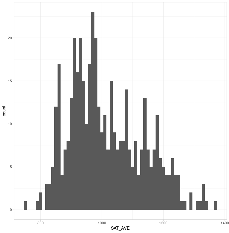
A histogram of SAT school average scores shows a right-skewed distributioncentered around 1000 with a standard deviation of 120.

           mean median     sd
SAT_AVE 1014.82    986 119.91

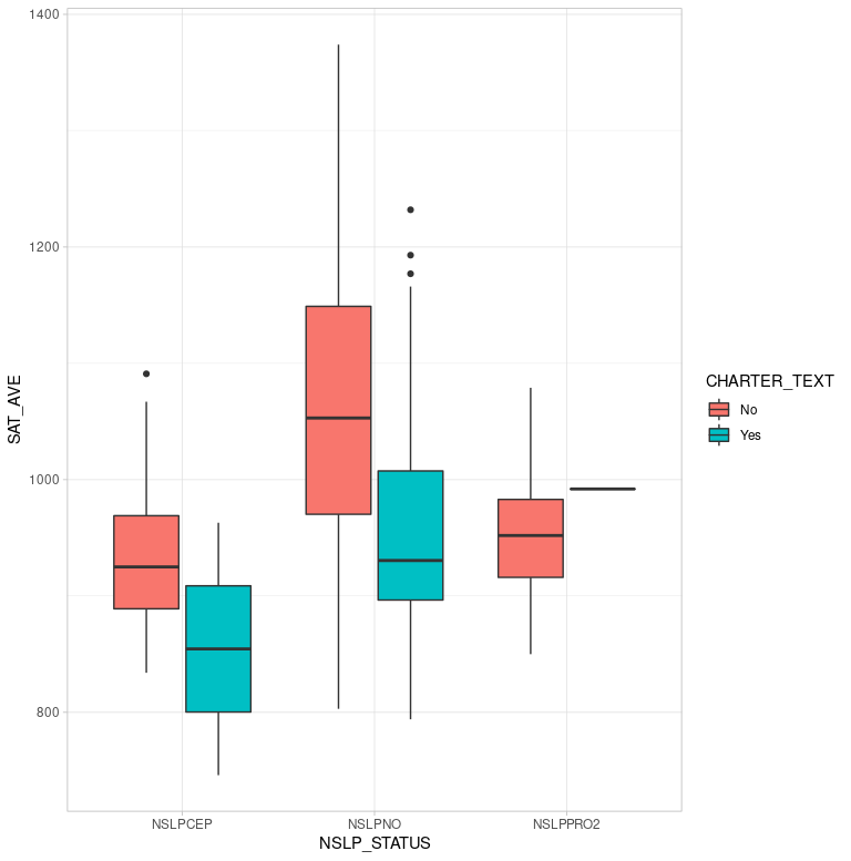
Boxplots of charter versus non-charter schools disaggregated by federal assistance through the National School Lunch Program (NSLP_STATUS) shows similar performance bands. Schools receiving aid (NSLPCEP n=75) look to have lower performance than schools not receiving aid (NSLPNO n=346). Another hypothesis to test is that from the chart it appears that charter schools perform lower than non-charters on the SAT.

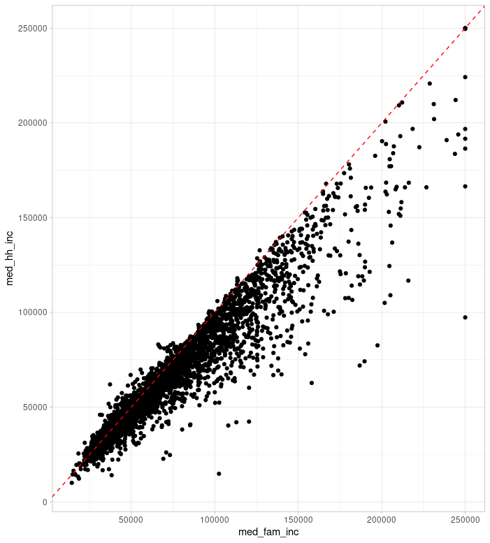
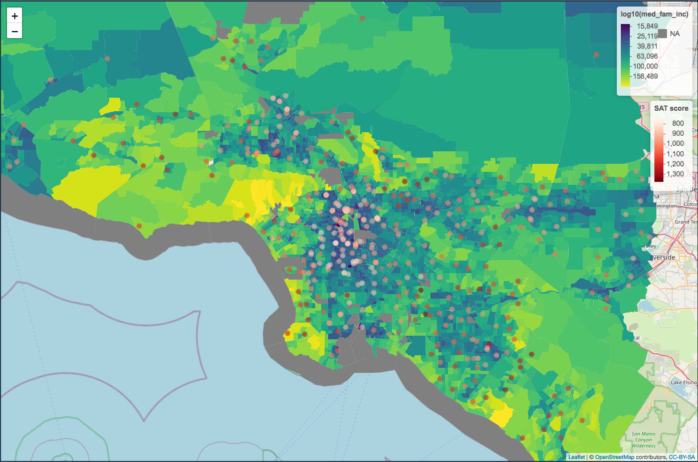
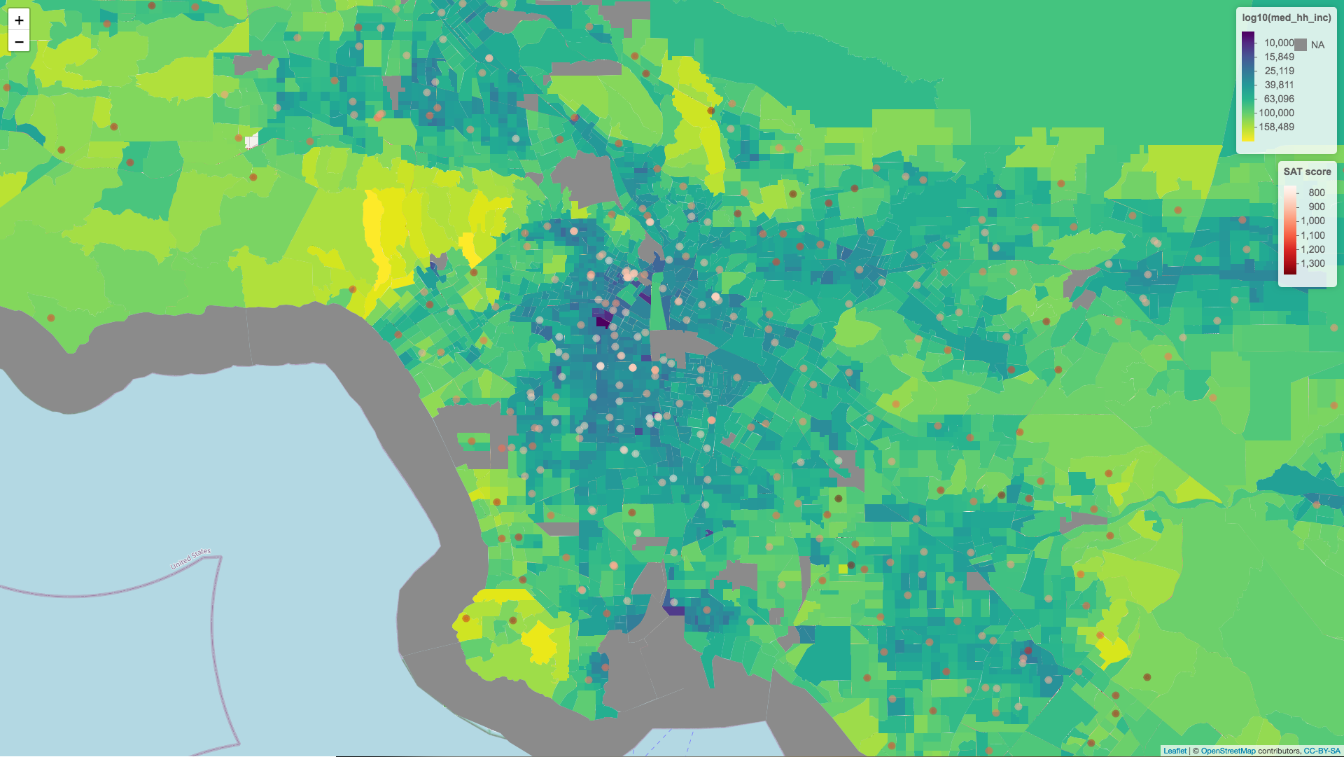
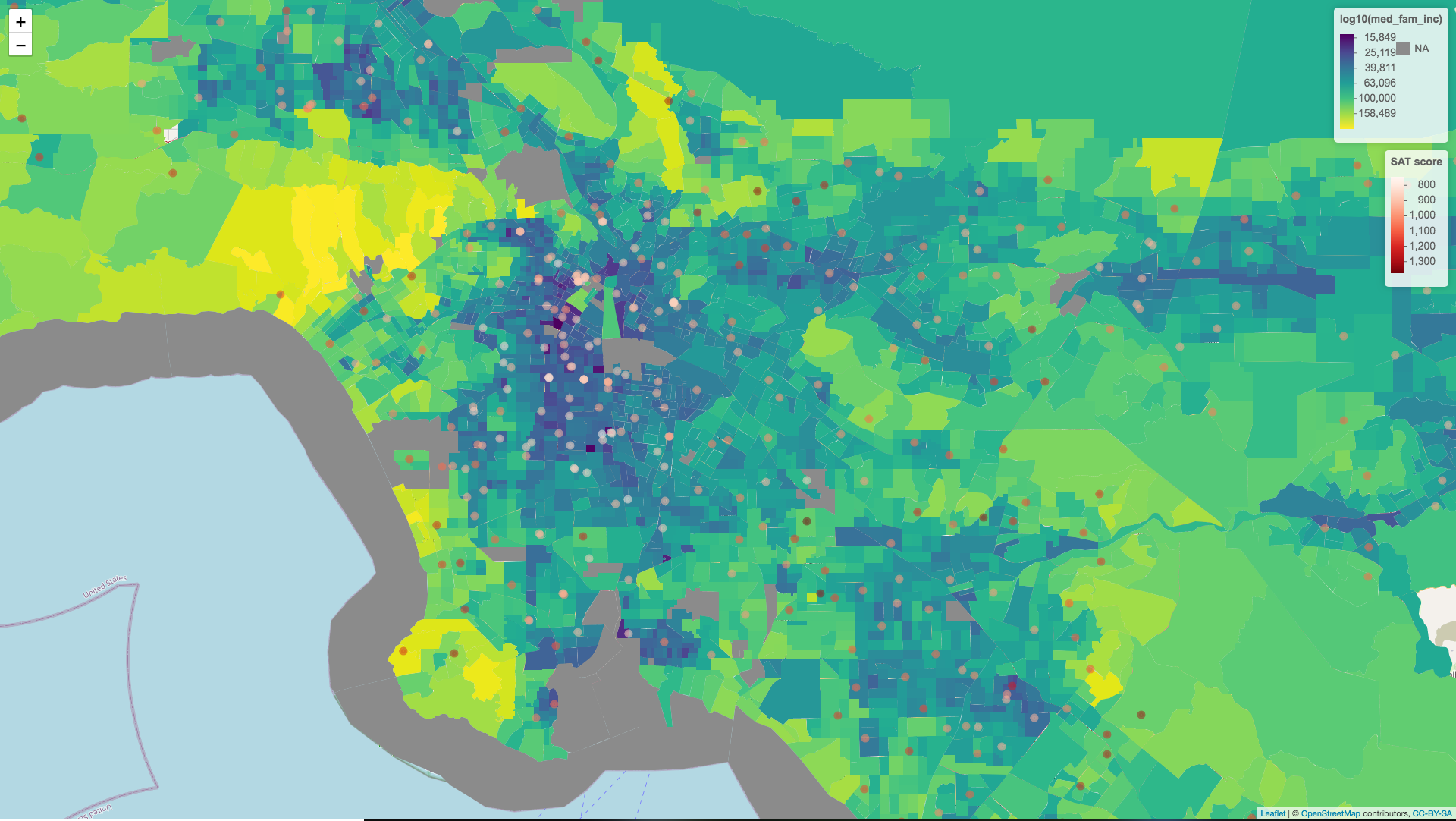
Median household income and median family income is another story. Since many families are seperated we can see that family income is often higher than household income. For the purposes of analysis we can see which of these variables more closely models the variation seen in SAT scores, but for the purposes of the image at the top of this post I was most interested in which variable created a more compelling visual. Note how family income creates darker regions in the poorer urban centers.

Analysis

I selected numeric demographic features to look at correlations with average SAT scores.

Result 1

Result 2 ANOVA? ANCOVA? GLM?

Result 3

__ % of the variation in SAT scores is explained by median household income of the census tract the school is in. Correlation is not causation, but it does give one pause to consider why this might be true.

the data is old. SAT 2016 and Census 2010. We can get new shapefiles, https://www.census.gov/geographies/mapping-files/time-series/geo/tiger-line-file.html

newer census data? https://data.census.gov/cedsci/

https://www.census.gov/library/stories/2018/10/opportunity-atlas.html looks interesting with opportunity bargains.

kop _crushton